Haldane’s Dilemma
In 1957, J.B.S. Haldane, a population geneticist and evolutionist, published the paper, "The Cost of Natural Selection", which defines a mathematical model for the spread of a rare, beneficial mutation through a population until it reaches “fixation” (i.e. it exists in virtually the entire population). His model shows that a large number of deaths must occur in the non-mutant carrying population before the new mutation reaches fixation. In species with low-birthrates, it means that new mutations accumulate slowly. His model has been used by creationists to argue that there is an upper limit on the number of beneficial mutations that could have reached fixation in the human lineage over the past few million years. Further, they argue that this number of mutations is insufficient to explain human capabilities above their primate ancestors. However, there are several situations which can dramatically lower the substitution cost of new mutations in a population, and thereby, increase the rate at which beneficial mutations can accumulate within a species. Two of those situations are: geographic separation, which can reduce the substitution cost to less than half it’s normal value, and simultaneous selection on multiple attributes, which can reduce the substitution cost well below 10% of its normal value.
Haldane’s Model
Haldane’s model starts with a population of organisms. Some change in the environment occurs (a new predator, a climate change, disease, etc) which lowers the survival rate of the population. A small number of organisms have a mutation which maintains it’s survival rate despite the change. As the animals lacking the beneficial mutation die as a result of this new selection pressure, the frequency of the beneficial mutation increases in frequency, until it becomes fixed in the population (i.e. it exists in virtually all organisms in the population). The spread of the beneficial mutation takes time, however, and the number of animals that die specifically because they lacked the beneficial mutation is defined as the “substitution cost”.
In order to use the model, first we define “s” (referred to as the selection coefficient). We define the survival rate of the organisms with the beneficial mutation as 1.0 (i.e. 100% survival). We define survival rate of the rest of the population as 1-s, where s is between 0 and 1. If we set s=0.1, the survival rate of the population lacking the beneficial mutation would be 1-0.1 = 0.9 (90% survival). We define “p” to be the proportion of the gene pool with the beneficial mutation. We must also define the population size “N”. 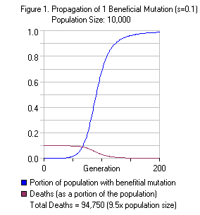 In this example, we’ll use a selection coefficient = 0.1 and population size = 10,000. Haldane assumed that the beneficial mutation would initially exist at some background level in the population, and used a p-value of 0.00005 (for dominant mutations in diploid organisms, this is equivalent to 1 copy for every 10,000 organisms). Because we use a population size of 10,000 in this example, the beneficial mutation exists in only one organism. Each generation, selection pressure will eliminate 10% of the organisms lacking the beneficial mutation. Initially, a single round of selection (one generation) will eliminate approximately 1000 of the 9,999 organisms lacking the beneficial mutation. These deaths are counted as part of the “substitution cost” of the new mutation. In contrast, 100% of the organism(s) with the beneficial mutation survive. We assume a stable population size, so in the first step selection pressure kills 1,000 organisms, the population drops to 9,000 and rebounds to 10,000 individuals in the next generation. This increases the proportion of the beneficial mutation from 0.0001 to 0.0001111 (an increase of around 11%). Repeating this procedure over and over until the beneficial mutation reaches fixation in the population requires hundreds of generations. In the long term, around 95,000 organisms die as part of the substitution cost of the beneficial mutation. As a proportion of the population (10,000), this is 9.5x. Figure 1 on the right shows the spread of the mutation through the population over the course of 200 generations along with the
|
||||||||||||||
Provided that we follow Haldane’s assumption of an initial p value of 0.00005, then the size of the population is irrelevant to the number of deaths as a proportion of the population size. In other words, a population size of 1,000 needs 9,475 deaths (9.5x the population size), and a population of 1 million needs 9.475 million deaths (9.5x the population size) to drive an mutation to fixation within the population. The selection value “s” makes a small difference in the number of deaths required to drive an mutation to fixation, but it doesn’t have a large effect unless s approaches 1 (see Table 1).
Haldane’s model can be used to calculate 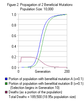 the effects of multiple selection pressures and mutations at the same time. In the situation where two independent selection pressures operate on a population at the same time, the deaths are nearly nearly cumulative. For example, let’s reproduce our previous example, but this time, we introduce a second selection pressure in the 10th generation and a second beneficial mutation (which affects an entirely different gene). The selection coefficient of this second selection pressure is 0.1. Figure 2 illustrates this situation. Note how, at the beginning of the chart, the number of deaths jumps from 0.1 (10% of the population dies) to 0.19 (19% of the population dies). This is because each selection pressure kills a portion of the population and their effect is compounded. In this case, 90% of the population survives the first selection pressure, and 90% of those survivors survive the second selection pressure - 81% survive both selection pressures. Note that the total number of deaths in Figure 2 is exactly twice the number of deaths in Figure 1.
Lowering the selection coefficient reduces the number of deaths in each generation, but increases the number of generations until the mutation reaches fixation. (Lower coefficients also produce slightly higher death tolls in the long term.) For example, a selection pressure with s=0.05 will cause half as many deaths per generation as one with s=0.10, but it requires about twice as many generations to bring the mutation to fixation. Over a period of, say, 200 generations, a population might be able to handle two sequential pressures of 0.1 (each one lasting around 100 generations), or two simultaneous pressures of 0.05 (each lasting the entire 200 generations). Both situations cause similar death rates (around 10%) over the period of 200 generations, and both situations would result in two beneficial mutations becoming fixed at the end of the time period. Attempting to add more selection pressures to a population causes a population decline (or collapse). What Haldane’s model shows is that there is a limit to the number of traits that can be driven to fixation over a specific period of time (assuming that population levels remain stable). Beneficial mutations can become fixed in a population much faster if the selection coefficients are very high (say 0.75+). However, when selection coefficients are high, it can cause population collapse in species that produce small numbers of offspring per generation.
This situation is not problematic for organisms that produce large numbers of children (e.g. bacteria, viruses, insects), because they can loose significant numbers of their offspring and still maintain stable population numbers. However, animals which have fewer numbers of children (for example, primates) cannot afford to lose too many children to selection pressure or else the population declines (perhaps to near-extinction levels), and requires a number of generations to recover when that happens.
One Beneficial Mutation every 300 Generations
So, how many beneficial mutations can be fixed in a population over a specific period of time? Haldane believed that selection pressures on larger, slow-reproducing organisms (primates, whales, elephants, etc) rarely culled more than 10% of the population of a generation. (This means, for example, that in a population where organisms produce 3 children per generation, selection pressures would typically cull fewer than 0.3 children.) Limiting selective deaths to 10% of each generation, we would calculate that one beneficial mutation could reach fixation every 100 generations. However, the previous calculations only model the spread of one dominant mutation. Haldane assumed that new mutations would be a mixture of dominant and recessive mutations. Recessive mutations have a higher substitution cost than dominant ones (up to 10x the cost), and so he decided that, on average, one beneficial mutation would reach fixation every 300 generations in large, slow-reproducing organisms. Thus, 300,000 generations would be needed to explain the accumulation of 1,000 beneficial mutations. The creationist, Walter ReMine, author of Intelligent Design book “The Biotic Message”, has used Haldane’s model to argue that there is a limit on the number of beneficial mutations that could have accumulated over the past few million years. Using a time-period of 10 million years, and 20 years between generations, has claimed that the entirety of the beneficial mutations that could be fixed in humankind’s lineage over the past 10 million years amounts to at most 1,667 - i.e. 10,000,000 years / [ 20 years per generation * 300 generations ] = 1,667 fixed beneficial mutations. He claims, based on intuition, that this is far too few mutations to explain humanity’s capabilities. (In actuality, it’s unknown how many mutations are needed to explain humanity’s differences with our primate ancestors.)
Geography and Subpopulations
Haldane makes the assumption that the entire population undergoes selection pressure at the same time and with the same intensity. This assumption causes a great deal of additional deaths. In our original case (illustrated in Figure 1), the the beneficial mutation exists in just one organism. The beneficial mutation increases in frequency only because, each generation, 10% of the non-mutation-carrying population dies for lack of the mutation. When the beneficial mutation is rare, this means that the frequency of the mutation in the gene pool increases by only 11% each generation. It takes 22 generations for the beneficial mutation to expand from 1 organisms to 10 organisms. It takes another 22 generations for the beneficial mutation to expand from 10 organisms to 100 organisms (a scant 1% of the total population). This is why Figure 1 and Figure 2 show very little visible change in beneficial mutation frequency over the first 50 generations. Meanwhile, because selection is acting on the entire population, the selection pressure is culling nearly 10% of the entire population. Those first 44 generations, which are spent getting the beneficial mutation to 1% of the population accounts for nearly 44,000 deaths, nearly half of the total substitution cost.
If, on the other hand, we assume that selection pressure affects only a subset of the population, total deaths can be dramatically reduced. Imagine a scenario where a new predator enters an area (putting selection pressure on a subset of the population), or a small group of organisms moves to a new location and encounters selection pressure (e.g. a new predator, a colder climate in the mountains, etc). Let’s say that our subgroup is composed of 1000 organisms and that a beneficial mutation is present in this group which allows it to survive the new selection pressure better than the others. What is the death toll on the small subpopulation? If we use Haldane’s assumption of p=0.00005 (the subpopulation contains the beneficial mutation at the same frequency as the larger population), the mutation spreads through the population over the course of a hundred or so generations. But, because there are fewer organisms under selection (1,000 instead of 10,000), there is a smaller death-toll in total numbers. It still requires a cost of 9.5x the population size, but it’s 9.5x the size of the subpopulation (9,475 organisms) rather than 9.5x the entire population (94,750 organisms).
Now, after this mutation has reached fixation in this subpopulation, let’s say that the selection pressure affects the entire population (all 10,000 organisms). Let’s also say that the subpopulation interbreeds with the rest of the population, thus allowing the beneficial mutation to propagate into the rest of the population. What’s the death toll of “phase 2” of this scenario? In essence, it mirrors the situation in Figure 1, except that we start out at generation 66 (where 10% of the population already has the mutation). This allows us to skip past the first 66 generations where the death-toll in Figure 1 was already ~64,000 organisms, and replace it with a death toll of merely 9,475. Thus, the total selective deaths drops from around 95,000 organisms to 40,000 (i.e. 4.0x the total population size). This scenario cuts the substitution cost by nearly 60% of its originally calculated value. Lowering the substitution cost means that the species can accumulate beneficial mutations at a faster rate because they have to “pay” for fixation with a fewer number of deaths.
By making this scenario more fine-grained, we could lower the substitution cost even further. For example, instead of jumping from 1,000 organisms to 10,000 organisms, the selection pressure could move from region to region, each containing a subpopulation, and the mutation could be passed from one region to the next through interbreeding. It seems quite likely that a species spread over a large area would experience this kind of situation involving different selection pressures (because of varying predators, disease, or climate). When paired with interbreeding across groups (allowing for the movement of the beneficial mutation), that situation lowers the substitution cost of an mutation below the value normally calculated by Haldane’s model.
Concurrency
Under Haldane’s Model, each beneficial mutation has to pay the full substitution cost. This makes sense under certain conditions. For example, if each beneficial mutation affects only one feature (e.g. the survival rate of the organism against one particular disease), then multiple diseases would create multiple independent selection pressures.
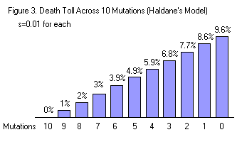 Consider a situation where there are ten different selection pressures and ten (corresponding) beneficial mutations (shown in figure 3). We’ll say that the selection coefficient for each of them is 0.01 (in each generation, 1% of the non-mutant population dies for lack of the mutation). In this case, organisms with 0 beneficial mutations have the highest death rate - nearly 10% per generation. Organisms with all ten beneficial mutations have a death rate of 0%. In order to bring all 10 mutations to fixation requires a (long term) death toll of more than 95x the population’s size (9.5 x 10 mutations), and approximately 1000 generations.
In this case, the selective deaths occur across virtually the entire population. During the first few hundred generations, the majority of the population has 0 beneficial mutations, and a minority has 1 or more beneficial mutations. Despite the fact that the organisms with 1 beneficial mutation are in the top 50 percentile of fitness, they have a survival rate of only 1% better than organisms with 0 beneficial mutations. Even organisms with 9 mutations (which may be much more fit than the majority of the population), are being selectively culled even though a 90% of the organisms with 0 beneficial mutations survive. In other words, when we apply selection deaths this way, it’s very inefficient because it kills some of the fittest organisms while leaving many of the least fit alive.
|
||||||||||||||||||||||||||||||||||||||||||
Truncation probably doesn’t happen very often in the real world. However, any selection model that skews deaths towards the least fit organisms will increase the rate that beneficial mutations spread through a population and reduce the substitution cost below Haldane’s 9.5x value. For example, 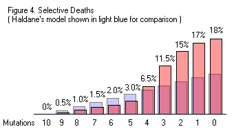 if selective deaths occurred similar to the rates shown in Figure 3, the rate of fixation would be faster than Haldane’s and involve a lower substitution cost. In the case where each of the 10 mutations exist in 50% of the population, a single round of selection under Haldane’s model would increase the frequency of each beneficial mutations from 50% to 50.21%. Using the selective death rates in Figure 4, that increase would be from 50% to 50.51%. Both cases would involve the deaths of 5% of the entire population, but Figure 4 results in the subsequent generation taking a bigger step towards the “ideal” population where all 10 mutations have been fixed.
This type of skewing can occur under certain conditions. For example, in cases where animals are in direct competition with each other, either through sexual selection or fighting (as with bucks), or there is a predator-prey relationship that results in one segment of the population being disproportionately killed. If our ten beneficial mutations were present in a population of gazelle, and the mutations enhanced the organism’s ability to flee from predators (lions, cheetahs, etc), then the slowest animals (those with the fewest beneficial mutations) might be killed in a pattern more similar to Figure 4 than Haldane’s selection model.
Additionally, if these mutations affected generalized health, it could also affect an organism’s reproductive success and survival. If some mutations affected the organism’s ability to fight off parasites and disease, other mutations increased the organism’s ability to capture prey, then organisms with the highest number of beneficial mutations would appear healthier (both better fed and with fewer health problems) than organisms with fewer beneficial mutations (which may appear sickly and weak - although still alive). If organisms chose to mate with the healthiest members of their population, then organisms with fewer beneficial mutations might suffer greatly in the competition for mates. This type of selection would skew reproductive success towards the healthiest members of the population and away from the unhealthiest (which is correlated with fewer beneficial mutations). This type of selection would bring mutations to fixation much faster than under Haldane’s model.
Consider a model where a population of organisms is split into five groups, each containing 20% of the total population. The top group contains the organisms with the most beneficial mutations, the second group contains organisms in the top 20th-40th percentile, and so on. Starting with the top group, we assign birth rates of 2.5, 2.25, 2.0, 1.75, and 1.5 (for the bottom group). This situation resembles the way an organism might do better reproductively if they are the best of their species versus the worst of its species. If organisms tend to mate with the best of its species, this type of pattern would be expected.
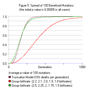 Figure 5 shows how 10% Truncation selection compares to two different group-birthrate methods assuming 100 beneficial mutations in the population. Like the Truncation model, the group-birthrate model allows fixation without paying the full substitution cost. Using birthrates of 2.5, 2.25, 2.0, 1.75, 1.5 children, 100 mutations are brought to fixation (p>0.95) in 335 generations. This is an average of 0.30 mutations per generation. In contrast, Haldane’s model allows for an average of 0.01 mutations fixed per generation, and would bring only 10 mutations to fixation within 1000 generations. Even when using milder group birthrates of 2.2, 2.1, 2.0, 1.9, 1.8 children, 100 mutations can be brought to fixation in 834 generations; an average of 0.12 mutations per generation. (Note: The second birthrate model involves an unused reproductive capability of 10% of the population each generation, which is the same 10% value Haldane estimated in his calculations.)
Using higher numbers of mutations and more elitist selection (larger reproductive bonuses for the best of the species, bigger penalties for the worst of the species), it’s possible to increase the fixation rate to even higher levels. For example, using group birthrates of 4, 3, 2, 1, 0 children, and 265 initial mutations, it’s possible to bring 265 mutations to fixation in 132 generations - a rate of more than 2 mutations fixed per generation, or 200 times the rate calculated by Haldane’s model.
Table 3 shows the number of generations required to bring X mutations to fixation. For example, under a the 2.5, 2.25, 2.0, 1.75, 1.5 Group Selection model, and 100 initial mutations, 100 mutations would be brought to fixation in 335 generations, which is an average of 0.30 mutations fixed per generation. (For comparison, keep in mind that Haldane’s model requires 100 generations per mutation, which is an average of 0.01 mutations fixed per generation.) So, 0.30 mutations fixed per generation is a 30-fold increase over Haldane’s “maximum” rate, and would turn ReMine’s “maximum” number of fixed mutations from 1,667 into 50,000!
|
||||||||||||||||||||||||||||||||||||||||||||||||||||||||||||
One difference between these models is that the fact that the birthrate model and truncation model gives a reproductive bonus to the best of the population and a reproductive penalty to the worst of the population. It is context-specific to the number of beneficial mutations an organism has relative to the rest of the population. For example, imagine a situation where there are ten beneficial mutations in existence, but we are early in our simulation, so all of them are rare. 80% of the population has zero beneficial mutations and 20% have one beneficial mutation. Under Haldane’s model, both groups have nearly the same number of selective deaths: ~10% for organisms with zero beneficial mutations, ~9% for organisms with one beneficial mutation. As a result, the frequency of these mutations in the population barely changes from generation n to generation n+1. More specifically, the children of organisms with 0 beneficial mutations makes up 79.82% of the next generation, and the children of organisms with 1 beneficial mutation makes up 20.18% of the next generation.
However, under a group-birthrate model of 2.2, 2.1, 2.0, 1.9, and 1.8, there is the same number of virtual deaths (i.e. unused reproductive capability) in generation n, but they are meted out differently. Under the group birthrate model, organisms with zero beneficial mutations suffer a slight reproductive penalty - having 1.95 children (equivalent to 2.2 children and 11.4% selective deaths), and organisms with one beneficial mutation have 2.2 children (equivalent to 2.2 children and 0% selective deaths). In this case, the children of organisms with 0 beneficial mutations make up 78% of the next generation, and children of organisms with 1 beneficial mutation make up 22% of the next generation. Under this model, selective deaths occur to organisms based on their beneficial-mutation percentile within the larger population. In contrast, Haldane’s selective deaths occur based simply on the number of mutations an organism has (regardless of how it compares to the rest of the population). In any population where sexual-selection occurs, it is unrealistic to ignore how an organism’s reproductive success varies based on how it compares to competition. But, Haldane’s model ignores this.
The fact that each beneficial mutation does not need to pay the full substitution cost means that these mutations can reach fixation much faster than assumed by Haldane’s model. This works provided that there is a mechanism to favor organisms with the most beneficial mutations. Sexual selection is one of these mechanisms, because organisms can favor a number of different traits at the same time and compare an organism’s traits to those possessed by other members of the same species. In the case of human ancestors, this would certainly be going on.
Haldane's model is still important in many situations, but has limited usefulness when trying to explain the total number of beneficial mutations in the human lineage. Many Creationists, on the other hand, believe it is the only model that explains mutation fixation, and use its slow pace and heavy death toll as evidence that the human evolution could not have happened within a realistic amount of time. Using hard numbers like “1,667” and phrases such as “evolutionary speed limit” are entirely incorrect and creates a false sense of concreteness. There are mechanisms that work much faster than Haldane’s model. The number of beneficial mutations that can be fixed per generation in the human lineage is much less dependent on Haldane’s model, and much more dependent on the rate at which new beneficial mutations are produced, and exactly how those mutations affect reproductive rates, survival rates, and their context within the larger population’s gene pool.
Creationist Claims and Counterclaims:
Walter ReMine says:
My book had the ambitious goal of teaching this cutting-edge subject to the ordinary person. I therefore began my discussion with an uncomplicated scenario for tutorial purposes. I discussed an ape-human-like species, with:
- an effective generation duration of 20 years
- a population-size of 100,000
- each and every generation receives a new exceedingly beneficial mutation with selection coefficient s=1 (that is, the previous genotype immediately vanishes)
- the substitution is completed in one generation, and the cycle is ready to repeat again each and every generation
- given 10 million years, or a total of 500,000 generations
— for a grand total of 500,000 substitutions.
This scenario is highly unrealistic in favor of evolution, but it is useful for teaching the basic parameters of the problem and how they interact. Such as the role played by the mutation rate, the selective value of the mutation, the population size, and of course the required reproduction rate (which is a central parameter), plus how these limit the number of substitutions. The discussion rhetorically raises questions to get my readers thinking in new terms. Once I teach the fundamentals, I move to a more realistic scenario — Haldane's — where one substitution occurs every 300 generations, for a total of 1,667 substitutions over the same era.
ReMine is arguing several points in this section: (1) maximum possible fixation rate for all species (including fast-reproducing organisms) is 1 beneficial mutation per generation, and (2) because humans are a slow-reproducing species, the actual fixation rate in humans is well below the “1 beneficial mutation per generation” value. Both of these points are false because ReMine (and Haldane, on whom he bases his ideas) completely ignores the power of concurrency. Not only is it possible to bring more than one mutation to fixation per generation in fast-reproducing organisms, but, under certain conditions, it’s even possible to do this in slow-reproducing organisms, such as humans.
In one example, I used 265 initial beneficial mutations and a 4-3-2-1-0 selection model, and the result was an average fixation of over 2.0 mutations per generation. This was not a miscalculation. Here’s a simple example to show how it’s possible to bring more than one mutation to fixation per generation.
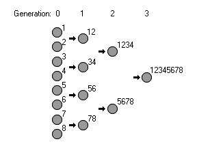 In this example, we start with 8 sexually reproducing organisms. Each of them have one unique, beneficial mutation. (The mutation which the organism has is shown by a number to the upper right of each organism.) They produce a number of children, but we only keep the best ones (the less-fit offspring are not shown in this illustration). Those best offspring go on to produce the next generation. In the example shown on the right, we can fix 8 beneficial mutations in 3 generations. In fact, under this selection method, the fixation of mutations occurs at an exponential rate. Now, this scenario is unrealistic for slow-reproducing organisms because it requires that the organisms have huge numbers of offspring. Huge numbers of offspring is necessary because we want children that contain the best of each parent, but it’s statistically unlikely for a child of two parents who each have four unique mutations to get all eight beneficial mutations (statistically, it’s 1 in 256). However, even if we weaken the model so there are fewer children born and we allow the not-quite-perfect organisms to reproduce, we can still get fast fixation of mutations - not as fast as in this illustration, but still faster than 1 per generation. Assuming we start with only 1 beneficial mutation per organism, then under ideal conditions (unrestrained birthrates, harsh selection), we can fix [2^(generations)] mutations per generation. This would allow fixation of 256 mutations in 8 generations (a rate of 32 mutations fixed per generation). But, because we are working under much milder conditions (as illustrated in the differential birthrate model earlier), we see lower mutation fixation rates, such as 0.3 or 0.12 mutations per generation. It’s the mixing of mutations that occurs in sexually reproducing organisms that allows this fast fixation to occur; 1 beneficial mutation per generation is most definitely not the ceiling on fixation.
Additional Information:
The Cost of Natural Selection, JBS Haldane
On the Biological Significance of the Cost of Gene Substitution, Joseph Felsenstein